Approximation models

Warning

This part may be more mathematics focused. If you simply want to grasp the intuition behind deep learning, feel free to skip the section.

What is an approximation model?

Mathematically speaking, an approximation model approximates (but may never be) the output function. For example, we can approximate \( 0 \) with the function \( \frac{1}{x} \). When \( x \rightarrow \inf \), the function \( \frac{1}{x} \) gets very close to \( 0 \). Notice that \( \frac{1}{x} \) can never become \( 0 \) no matter how big \( x \) gets, but \( \frac{1}{x} \) gets close enough to \( 0 \) that we don’t care about that anymore.

A machine learning model is no different. Taking the cat/dog differentiator for example. Since mapping from images and labels can be seen as a function’s inputs and outputs, if we can use a model to approximate the mapping, and do a well enough job, then the model is essentially a good appproximation model to the function that maps from cat images to cat labels and dog images to dog labels.

How well can a model approximate?

Well, it’s proven that a model can be as accurate as it wants, provided enough parameters.

Suppose we have a function mapping from \( x \) to \( y \). With such a simple function, we can plot it on paper.

%matplotlib inline

import numpy as np
from matplotlib import pyplot as plt

x = np.arange(60000) / 10000
y = np.sin(x)
plt.plot(x, y)
plt.show()

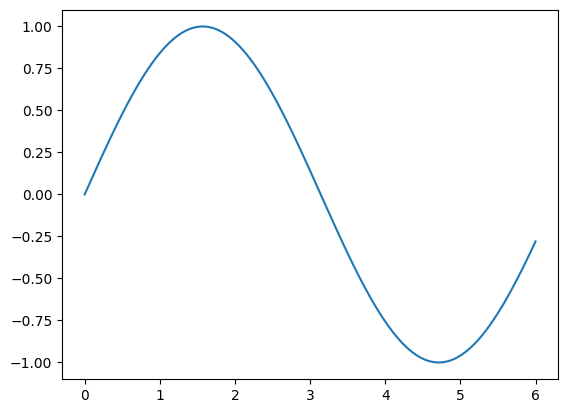
You see a sine wave right? However, this sine wave isn’t really smooth! It consists of a lot of little segments that are just too small to see. Let’s scale up a bit.

x = np.arange(12) / 2
y = np.sin(x)
plt.plot(x, y)
plt.show()

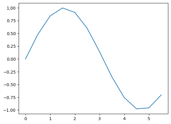
See how the shape is approximated by a lot of line segments? Here’s the deal, we could approximate any function with line segments, as long as we have enough of it. A machine learning model basically works the same way, creating truly complicated approximations to real world functions (like cat images to cat labels) by using a lot of simple functions (activation functions, more on that later).

Now you should use your imagination. For higher dimension \( x \), we can still think of it as a “line”, just that this line is high dimensional. If \( x \) is 2D, then this line is a surface. For higher dimension though, you’ll have to use your imagination.

Why deeper is better?

Suppose that we have a simple model where a neuron (a node in a layer) makes a decision: is the number bigger than a threshold? In other words, each neuron n separates the numbers into two intervals, bigger than n, or smaller than n.

We have two models:

1. One layer with three nodes.

2. Three layers with one node each.

For model 1, it could separate all possible inputs (numbers) into 4 intervals (because each neuron separates the current interval in half.) For model 2, because every neuron depends on the neuron comes before it, it could separate all possible inputs (numbers) into 8 intervals (2 to the power of 3).

8 is bigger than 4!

The reason deeper models perform better follows the same reason.