Gaussian Mixture Model

Note

We will refer to Gaussian mixture model as GMM in this section.

Note

We will refer to Gaussian distribution as simply Gaussian in this section

What are GMMs?

A GMM uses many Gaussians to approximate the probability of events. With the model, you can guess at what place the new event will happen.

When to use GMMs?

GMMs are good for creating input. Because it models a distribution by combining several Gaussians, it is capable of generating sample data from that distribution. A GMM is also super useful in that it uses minimal parameters, one average vector \( \mu \), and one covariance matrix \( \sigma \) for each Gaussian. And that’s it! Usually, it’s used when we want a fast way to have a relatively good model.

Why GMMs use Gaussians?

We all know gaussians right? The one that looks a bit funny, like a pile of slime. It’s also called normal distribution, because of how common it is in modelling the real world. That’s the reason for many cases using a few Gaussians in a GMM will produce sufficely good results. Gaussian also has a special property, that it can approximate any distribution given enough Gaussian distributions, which is also the reason it’s used in GMM.

How does GMM look?

We said that GMM is basically a mix of multiple Gaussian distributions. So how does this new distribution look like?

%matplotlib inline

import numpy as np
from matplotlib import pyplot as plt

def gaussian(x, mean, stddev):
    exponent = - (((x - mean) / stddev) ** 2) / 2
    numerator = np.exp(exponent)
    denominator = (stddev * np.sqrt(2 * np.pi))
    return numerator / denominator

# Choose number of gaussians
num_gaussians = 6

means = np.random.randn(num_gaussians)
# stddev should be larger than 0
stddevs = abs(np.random.randn(num_gaussians))

# weights should sum to 1
weights = abs(np.random.randn(num_gaussians))
weights /= weights.sum()

x = (np.arange(-200, 201) / 20).tolist()

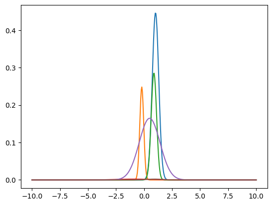
for n in range(num_gaussians):
    y = [gaussian(x[i], means[n], stddevs[n]) * weights[n] for i in range(len(x))]
    plt.plot(x, y)

plt.show()

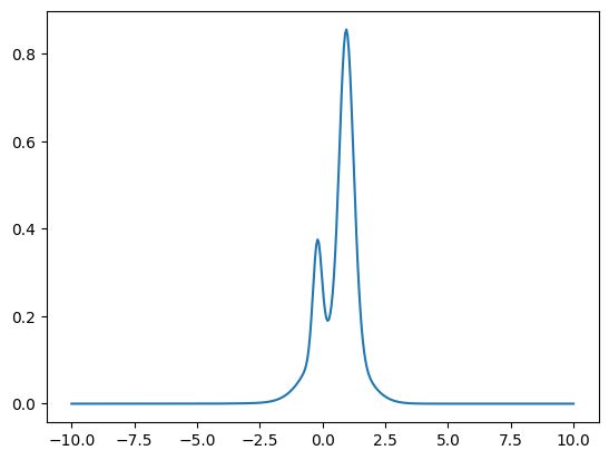
The sum of Gaussians is the look of the new distribution.

y = [0] * len(x)
for n in range(num_gaussians):
    for i in range(len(x)):
        y[i] += gaussian(x[i], means[n], stddevs[n]) * weights[n]

plt.plot(x, y)
plt.show()